Lonpos Puzzle Solver

I have a little puzzle that has sat on my desk for years. While I’ve never spent the time necessary to solve it myself, something about the simplicity of it made me never throw it away.

The fact that I’d never solved it before bugged me though, and so with one weekend free I decided to finally solve the puzzle… completely. According to the outside of the box the puzzle has $21,200$ solutions, so I attempted to find them all.

Most people will have seen this (or a similar) puzzle before; you have a set of different tetromino like pieces you’re able to place in a grid. There is just enough pieces to completely fill the grid and so the difficulty is finding the positions and rotations that fit all the pieces in.

The algorithm

During this project I was taking a computer algorithms paper at University, so I naturally decided to solve the problem with some of the methods we’d learned. Specifically I wanted to create a depth first search tree (DFS). This prioritises finding solutions as fast as possible.

If you haven’t heard of a DFS algorithm before it is simply a way of prioritising which decisions to make. A common problem in algorithm design is that often the algorithm must make a choice of what action to take. There usually isn’t a “right” choice to make and instead both need to tried and tested at some stage. So which action should be taken?

This is exactly the problem our algorithm will have to face since it will have the opportunity of being able to place many pieces without one being the obvious “right” choice. Given $n$ pieces, the first piece placed could be any of the $n$ pieces (We need to try them all at some stage), then it would be able to then place any one of the $n-1$ pieces, then $n-2$ pieces and so on.

If $n=4$ then the tree of decisions would look like the following.

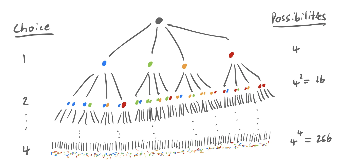
Each successive level is the state after taking that number of choices. If $k$ is the number of choices taken there are $n^k$ possibilities at that stage. The bottom of the tree are all the permutations of pieces with $n^n$ possibilities. For $n=4$ this is a manageable 256 possibilities, however the lonpos puzzle has $n=12$ pieces which means there are 8 trillion possibilities! But as these pieces could all be rotated and mirrored, which then influences the future placement of pieces, it could be interpreted that there are $n=12\times 4\times 2=96$ pieces leading to $2 \times 10^{190}$ possibilities… This is the number 2 followed by 190 zeros and is difficult to comprehend.¹

The need for a smart algorithm is clearly essential and the DFS algorithm gives us a way of navigating this tree to make sure that every valid branch has been tried and tested. As soon as a branch has been identified as invalid, then there is no need to check its descendants as they will be invalid too!

Zigzagging down the board, the algorithm will look for a gap and then place a piece down before continuing onto the next spot.

Eventually, the algorithm will encounter one of two obstacles

• Either the algorithm will run out of pieces to place which means the algorithm was successful, and we found a solution that fits all the pieces!
• Or, there will be no valid pieces left to place as no piece fits into the remaining gaps without overlapping some previous pieces.

Either way, the algorithm can go back up the decision tree until it finds the last decision it made with other valid choices left. Then it makes its second choice and continues along that branch until encountering another obstacle.

The nice thing about DFS is that it can be coded really easily by recursion² and a good way of thinking about recursion is as a black box that calls other black boxes. Imagine we have the following parts:

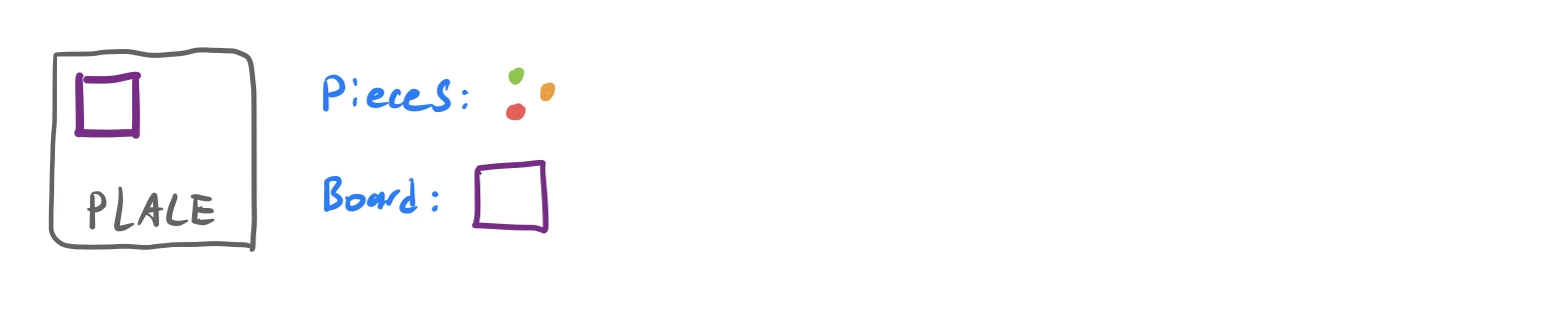
The box Place takes in a board and then attempts to place an available piece in a gap that it finds. Sometimes multiple pieces are possible to be placed and sometimes no pieces can be placed. The DFS algorithm would then work as shown.

Building the algorithm

Enough generics, let’s build the algorithm!

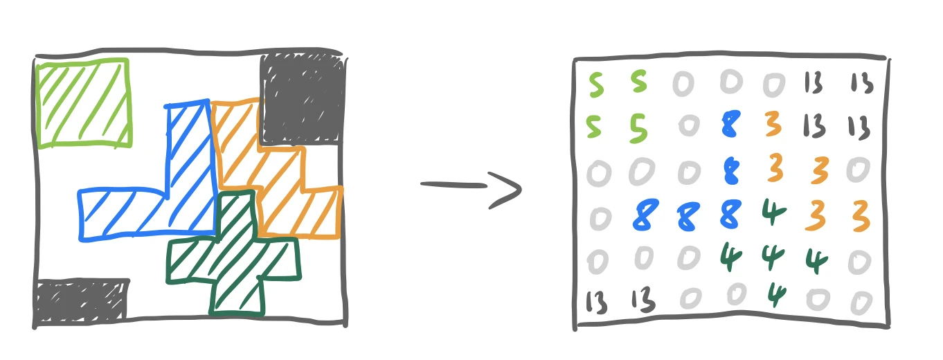
First we need to represent the board internally in the code. The easiest way of doing this is by encoding each piece by a number and placing these numbers in a matrix. We let $0$ represent empty space and $13$ represent the border of the puzzle where pieces cannot be placed (as the puzzle is not a square!). Numbers $1-12$ each indicate a specific piece corresponding to their location.

Strictly speaking we could just encode all “filled space” as just one number and the code would remain unchanged, but by doing it this way it is much easier to visualise the board.

The place function

Now we have to work out if the piece can be placed validly.

One way of doing this is to calculate the sum of the board and piece separately, and then calculate the sum of the board with the piece placed in it. Clearly if this sum is the same then the new piece only replaced 0s in the original board

if np.sum(board) + np.sum(piece) == np.sum(newBoard)

But this is slow and many steps are being repeated. Most of the board remains unchanged if a single piece is added, so calculating the total sum twice just slows things down.

A much faster way to do this is by use of masks so only the part of the board that is changed is summed. From the entire board we can select the region that the new piece would be placed in as view. Then we just need to compare the empty (locations corresponding to $0$) spots in view to where the piece is. If this sum is $0$, then there is nowhere that the piece overlaps with the existing board and so it can be successfully placed. Written in python this is

view = board[y:y + piece.shape[0], x:x + piece.shape[1]]
if np.sum(view[piece != 0]) == 0

Where x and y are the coordinates of the piece being placed..

The recursive loop

Now we need to create the recursive algorithm to complete DFS.

Most of the magic happens in this compute function in core.py, which has been stripped back in this version to show the main logic (61 lines down to 19!)

def compute( ... ):
    while j < board.shape[0]:
        while i < board.shape[1]:
            if board[j, i] == 0:  # find the piece that goes here!
                for generalPiece in pieces:
                    for piece in permuatations(generalPiece): 
                        possible, newBoard = place(board, piece, i, j)
                        if possible:
                            remaining = pieces.copy()
                            remaining.pop(generalPiece)
                            if len(remaining) == 0:  # Done (save it)! 
                                stats["solutions"].append(newBoard)
                            else:
                                compute( ... )  # keep trying...
                return stats["solutions"]  # unable to place any pieces
            i += 1
        j += 1
        i = 0
    return stats["solutions"]  # end of the tree

Here you can see the guts of the algorithm. The outer two while loops iterate over every spot in the board with coordinates (i, j) while the inner if statement checks to see if the current square is empty. It then attempts to place a piece in this empty spot.

For each empty spot, we have a choice of all the remaining pieces and for each piece we have a choice of all the different orientations that they could be in! These are tried systemically by the algorithm since it moves on if a piece was successfully placed but is not complete in the line compute( ...).

If there are no remaining permutations available to place then the for loops terminate and the runner returns to the parent for loop repeating with another available piece. This is how the algorithm is able to back up the tree and traverse another branch instead.

(These visualisations are generated live with the help of Blessings and some generic emojis)

This animation is slowed down, so it’s possible to see what the algorithm is doing but running it “headless” is significantly faster.

Run it

With the code complete the only thing left to do was run and wait. Not long later the algorithm terminated, and it was time for the big reveal: how many solutions had is found?

It returned exactly $21,200$ solutions. The same number as the outside of the box.

Satisfaction achieved.

It is quite uncommon that it’s possible to verify your solution, and even more uncommon to hit it exactly on the nose!

We end up with a list of valid board solutions in pre-order tree traversal order. To a loose extent solutions that are similar to each other are found next to each other.

Afterword

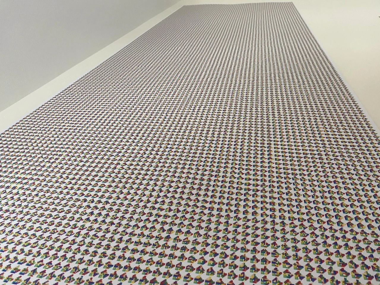
It’s a bit different playing with the puzzle now. The result of this image is that it is like having every possible checkmate printed out and stuck on your wall. No matter what game you play, no matter how creative you are, the game will always end up in one of those endings. Is there any point in playing?

Of course all the code is available on Github. Go check it out.

Next steps

As the code created is easily modifiable we could adjust the rules and see what occurs. It would be quite interesting to swap some pieces out for new pieces and see how the puzzle changes. Perhaps it would become easier with more solutions available, or phenomenally more difficult?

We are also not limited to this board shape. Perhaps other board shapes could allow more flexibility?

One thing I am searching for is a board and piece combination that only has $1$ solution instead of $21,000$ solutions. This is quite hard the difference between having $1$ solution and no solutions isn’t much. Often if the board is very difficult it has no solutions at all, and if it has one solution often many others are also possible. Striking a balance will be difficult…